Introduction Paper: Policy Gradient Methods for Reinforcement Learning with Function Approximation
Authors: Richard S. Sutton, David McAllester, Satinder Singh, Yishay Mansour
Vanilla Policy Gradient
In this post, I will introduce the simplest case of stochastic, parameterized policy. The objective goal is to maximized the expected return (here we consider finite horizon un-discounted return as example):
The gradient of policy performance, is called the policy gradient. In general, we call the algorithms that optimize the policy in this way the policy gradient algorithms. To optimize the process, usually we need an expression for the policy gradient that we can numerically compute, which contains two steps:
- deriving the analytical gradient of policy performance;
- forming a sample estimate of the expected value.
Now let’s see the derivation of a trajectory with the simplest form of the expression. First I have addressed some facts in deriving the analytical gradient, 
Combining them together, we can derive the first-order derivative of expected return as follows:

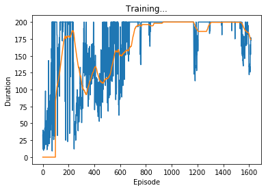
Example of Vanilla Policy Gradient Using cartpool From OpenAI Gym
import torch
import torch.nn as nn
import torch.nn.functional as F
from torch.distributions import Bernoulli
from torch.autograd import Variable
from itertools import count
import matplotlib.pyplot as plt
import numpy as np
import gym
import pdb
class PolicyNet(nn.Module):
    def __init__(self):
        super(PolicyNet, self).__init__()

        self.fc1 = nn.Linear(4, 24)
        self.fc2 = nn.Linear(24, 36)
        self.fc3 = nn.Linear(36, 1)  # Prob of Left

    def forward(self, x):
        x = F.relu(self.fc1(x))
        x = F.relu(self.fc2(x))
        x = torch.sigmoid(self.fc3(x))
        return x
# Plot duration curve:
# From http://pytorch.org/tutorials/intermediate/reinforcement_q_learning.html
episode_durations = []
def plot_durations():
    plt.figure(2)
    plt.clf()
    durations_t = torch.FloatTensor(episode_durations)
    plt.title('Training...')
    plt.xlabel('Episode')
    plt.ylabel('Duration')
    plt.plot(durations_t.numpy())
    # Take 100 episode averages and plot them too
    if len(durations_t) >= 100:
        means = durations_t.unfold(0, 100, 1).mean(1).view(-1)
        means = torch.cat((torch.zeros(99), means))
        plt.plot(means.numpy())

    plt.pause(0.001)  # pause a bit so that plots are updated
# Parameters
num_episode = 5000
batch_size = 2
learning_rate = 0.01
gamma = 0.99

env = gym.make('CartPole-v0')
policy_net = PolicyNet()
optimizer = torch.optim.RMSprop(policy_net.parameters(), lr=learning_rate)

# Batch History
state_pool = []
action_pool = []
reward_pool = []
steps = 0
for e in range(5): #num_episode

    state = env.reset()
    state = torch.from_numpy(state).float()
    state = Variable(state)
    #env.render(mode='rgb_array')
    #print(state)

    for t in count():

        probs = policy_net(state)
        m = Bernoulli(probs)
        action = m.sample()
        action = action.data.numpy().astype(int)[0]
        next_state, reward, done, _ = env.step(action)
        #env.render(mode='rgb_array')

        # To mark boundarys between episodes
        if done:
            reward = 0

        state_pool.append(state)
        action_pool.append(float(action))
        reward_pool.append(reward)

        state = next_state
        state = torch.from_numpy(state).float()
        state = Variable(state)

        steps += 1

        if done:
            episode_durations.append(t + 1)
            #plot_durations()
            break

    # Update policy
    if e > 0 and e % batch_size == 0:

        # Discount reward
        running_add = 0
        for i in reversed(range(steps)):
            if reward_pool[i] == 0:
                running_add = 0
            else:
                running_add = running_add * 1 + reward_pool[i] # gamma
                reward_pool[i] = running_add


        # Normalize reward
        reward_mean = np.mean(reward_pool)
        reward_std = np.std(reward_pool)
        for i in range(steps):
            reward_pool[i] = (reward_pool[i] - reward_mean) / reward_std

        # Gradient Desent
        optimizer.zero_grad()

        for i in range(steps):
            state = state_pool[i]

            action = Variable(torch.FloatTensor([action_pool[i]]))
            reward = reward_pool[i]

            probs = policy_net(state)
            m = Bernoulli(probs)

            loss = -m.log_prob(action) * reward  # Negtive score function x reward
            loss.backward()
        optimizer.step()

        state_pool = []
        action_pool = []
        reward_pool = []
        steps = 0


